Page 18 - Education and Inclusive Growth --Jong-Wha Lee Korea University
P. 18
164 ᐿၾආӉjԃٙɢඎ
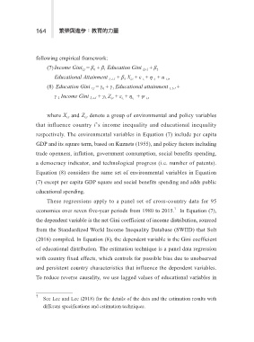
following empirical framework:
(7) Income Gini = β + β Education Gini I,t-1 + β
0
I,t
2
1
Educational Attainment I, t-1 + β X + ε i, + η t, + u i,t ,
5
i,t
(8) Education Gini I,t = γ + γ Educational attainment I, t-1 +
1
0
γ Income Gini I, t-1 + γ Z + ε + η + ψ i,t
2
3
t,
i,
i,t
where X and Z denote a group of environmental and policy variables
i,t
i,t
that influence country i’s income inequality and educational inequality
respectively. The environmental variables in Equation (7) include per capita
GDP and its square term, based on Kuznets (1955), and policy factors including
trade openness, inflation, government consumption, social benefits spending,
a democracy indicator, and technological progress (i.e. number of patents).
Equation (8) considers the same set of environmental variables in Equation
(7) except per capita GDP square and social benefits spending and adds public
educational spending.
These regressions apply to a panel set of cross-country data for 95
economies over seven five-year periods from 1980 to 2015. In Equation (7),
7
the dependent variable is the net Gini coefficient of income distribution, sourced
from the Standardized World Income Inequality Database (SWIID) that Solt
(2016) compiled. In Equation (8), the dependent variable is the Gini coefficient
of educational distribution. The estimation technique is a panel data regression
with country fixed effects, which controls for possible bias due to unobserved
and persistent country characteristics that influence the dependent variables.
To reduce reverse causality, we use lagged values of educational variables in
7 See Lee and Lee (2018) for the details of the data and the estimation results with
different specifications and estimation techniques.

